Solving TEAM30a with SMEKlib and Comsol

Comparing SMEKlib and Comsol

If you do electromagnetics, you’re certainly familiar with the TEAM workshop problems. Indeed, these problems are widely used to benchmark and validate simulation algorithms againt measurement data, and each other.

Here’s a case example – solving Problem 30a with SMEKlib and Comsol both.

Problem 30a

Problem 30a consists of a very simple induction motor; illustrated in meshed form below. The rotor consists of solid steel (grey, towards the center of the figure), coated with aluminum (cyan). The stator has six coils (red + green), separated by air (yellow). Finally, the stator has a thin yoke (again grey).

Now, the aim is to determine e.g. the voltages induced in the stator coils, and the resistive losses in the rotor.

Analysis

An asynchronous machine with a solid rotor is peculiarly simple to analyse. Indeed, since the motor is fully symmetric, the entire machine can be analysed in the stator coordinates (reference frame). The electric field (and currents) in the rotor can then be obtained based in the Lorentz force formula.

Alas, this type of analysis cannot be applied to machine with a slotted rotor. So far, it hasn’t been implemented in SMEKlib for this very reason. So, I opted for the more general approach, analysing the stator and rotor both in their respective frames. In other words, setting the frequency in the rotor equal to .

In this case, simulation accuracy takes a hit. Thus, the results won’t nicely match the measured ones listed on the TEAM website. However, this does not prevent us from comparing the results from two different software.

In this case, Comsol and SMEKlib. Comsol is well-known commercial FEA software, widely used in the industry. By contrast, SMEKlib is my open-source library (MIT license, so you can even repackage and sell it as long as you acknowledge me) for Matlab and Octave.

Soon, we’ll see how they turned out.

Comsol Model

I implemented to the induction machine problem in COMSOL. I don’t really know what else to say about it. If you want to learn Comsol, I’m not the best possible teacher.

SMEKlib Model

As far as machine simulations in SMEKlib go, this was remarkably simple. You can download the entire problem from the Github repository, under demos.

The demo_TEAM30.m file is the main simulation script. Additionally, there’s a set of simulated data exported from Comsol for comparison purposes.

The geometry was meshed in gmsh, based on the geometry created by the wonderful Mr. Jonathan Velasco. The gwrap wrapper for gmsh used in SMEKlib is quite new, so make sure you are using the latest version. If, for some reason you don’t have gmsh installed, you can simply comment out the line 25

gwrap_mesh(gmsh_path, geo_path);

in the main script, to use the pre-meshed geometry in the file Problem30a.msh.

Alright, that’s about it.

Let’s move on to the results!

Simulation Results

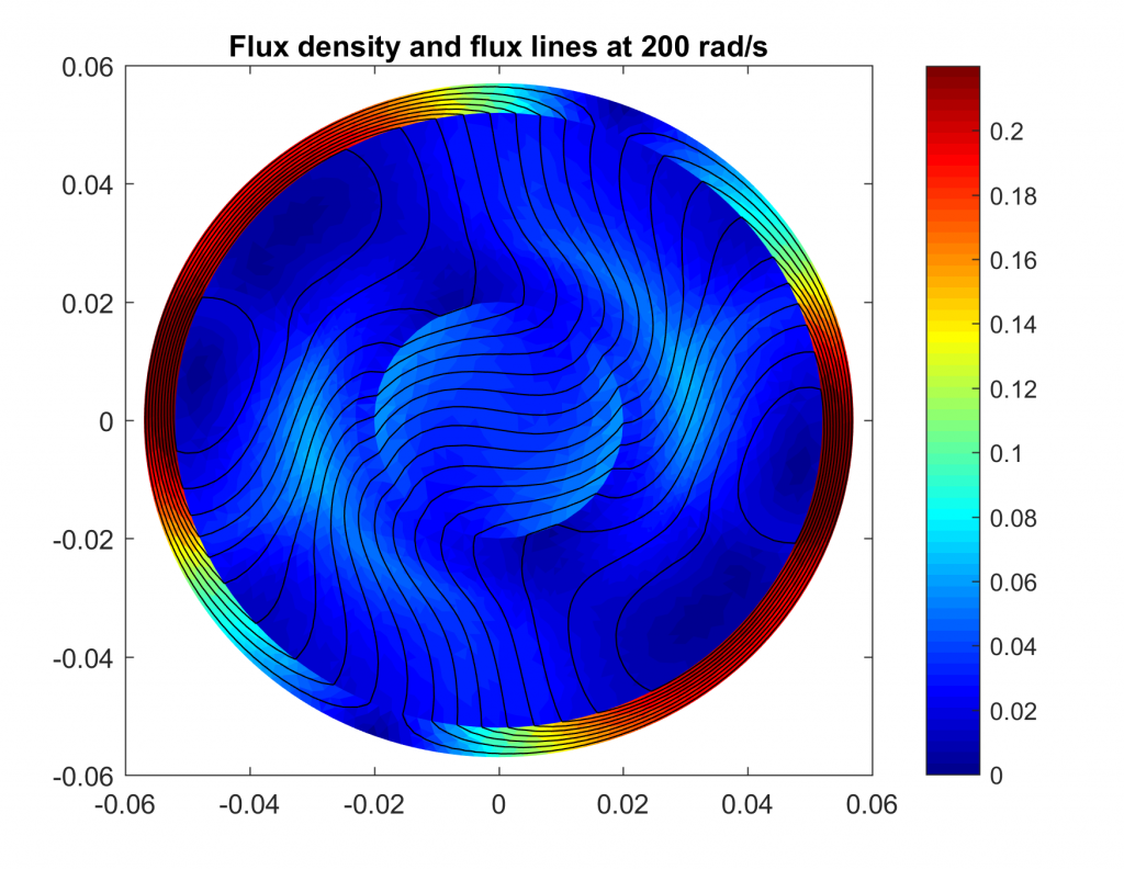
Everybody loves flux plots, so let’s begin with them. Below, the results from Comsol

followed by those from SMEKlib.

As you can see, they are quite close to each other. Lightly put. Of course, there are some deviations, but they can probably be attributed to different image processing used by Comsol.

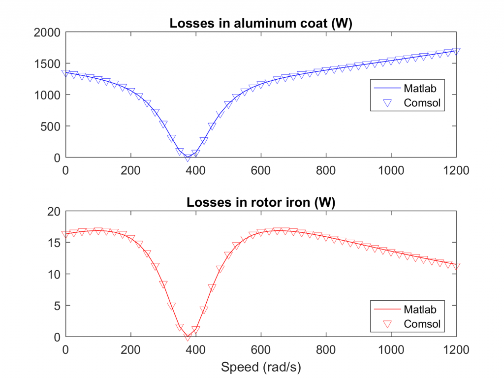
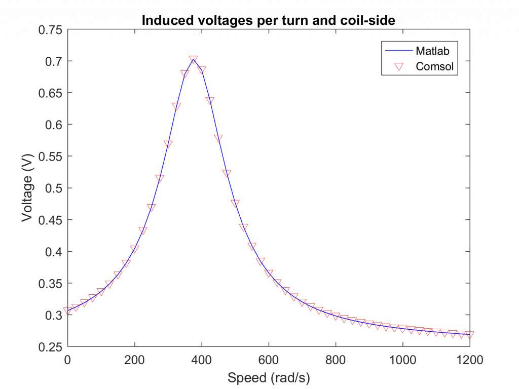
For closer analysis, I also plotted to losses in the rotor iron and aluminum both, as well as the torque and the voltages induced in the stator coils. The results you can find below.

As you can see, the results match very nicely. The differences between the rotor losses were well below 1 % throughout the entire speed range analysed. Torque was even better, with approximately 0.15 % deviations. Voltages differed somewhat more, roughly 2 % on average.

Computation times

Both models had roughly the same number of unknowns – 3005 in Comsol, and 3666 in Matlab. Despite this, there was a marked difference in computation times.

Indeed, Matlab solved all 49 operating points in 1.25 seconds. By contrast, Comsol took 6 seconds. That means SMEKlib was almost 5 times faster in this case.

Wait – There’s more!

Oh yeah, right! I also included a time-stepping simulation to the end of the simulation script. Nothing too interesting there, mainly to see how big an error the harmonic approximation causes in the current density.

You can check it out on your own in case you’re interested.

In any case, that’s all for now. See you in a while!

-Antti

Solving TEAM30a with SMEKlib and Comsol