Determining and Quantifying Sources of Uncertainty

Finding the sources of uncertainty

In my last post, I introduced to you uncertainty quantification. Simply put, uncertainty quantification (UQ) follows the propagation of random variations from some less-than-fully known input, to some interesting output. For example, how errors and deviations in the manufacture process influence the performance of the final product.

Finding the roots

Unsurprisingly, the first step in the process is determining what is introducing uncertainty in the first place. This questions has a simple answer: everything is. Think of it – nothing is certain, at least if you move to such precision levels where the Heisenberg uncertainty principle starts to have an effect. In practice, there’s no need to go even nearly that deep. Plenty can go wrong on the macroscopic level, too.

Answering the question in a non-idiotic fashion is harder. Everything might be uncertain, but not everything is uncertain enough to have a non-negligible effect. Picking the important factors may require multi-disciplinary experience and collaboration. Like – gosh – speaking to people! Horrifying!

Two categories for uncertainty

In all seriousness though, we need to understand the different parts and stages of the production cycle and their effect on the final product. What we are looking for can generally be classified as either uncertain material parameters, or uncertain geometry. With the former, a good idea might be to start with such parameters that you can find in your simulation model too – those are probably the most significant. A similar rule of thumb can be applied to the geometry, too, as long as you’re careful enough.

But as I mentioned earlier, all of these factors will be at least somewhat uncertain. Accordingly, the next step is to find the ones most likely to have a meaninful effect. In other words, we are beginning to determine:

• How large uncertainties are there in a particular parameter, or aspect of the geometry.
• How large of an effect we can expect it to have.

At this stage, very rough numbers are enough. Guesstimates such as “not at all” versus “a lot” are sufficient, as is getting some number correct to the nearest ten-fold. The actual quantification part comes later.

Talking to folks

Pooling the expertise of different people is the best way to get started, unless you already have a very good idea yourself. For instance, senior workers will certainly know if the paint finish of a certain motor family is prone to flaking after roughly two years. And an electrical engineer knows it has absolutely no effect on the motor performance. (At which a service engineer will cut in and remind us that it definitely has an effect on the motor lifetime under humid conditions.) Or, an electrical engineer might worry about the resistivity of the rotor bars. However, the manufacturer would probably convince them that this is not a problem.

But for electrical engineers, bearing or winding manufacture might be more interesting, for example. The former can introduce eccentricity to the rotor, which is then evident in the electromagnetic characteristics. And the latter ties nicely to my pet topic of circulating currents and other AC losses.

Anyway, talking to experts involved in different stages of the production cycle should give you a good idea on where to start. You’ll know what can be done in a precise fashion, and what can’t. Combine that knowledge with your knowledge about the expected significance of each factor, and you’re ready to move to the next stage.

What to quantify

By no you can probably guess that the next step is quantifying the uncertainty. For that purpose, we need to know both the what and how.

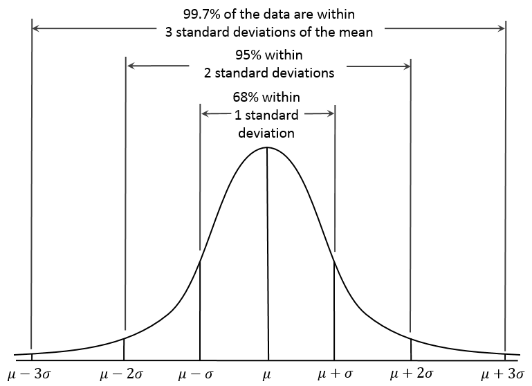
Let’s begin with the what. What are we quantifying, after all? Well, since we are dealing with a random variable, you might be inclined to suggest numbers such as the mean value and variance. Stuff from high school statistics.

And you’d be perfectly right to do so: they are important characteristics after all. Simply knowing the mean value can get us started, and knowing the variance might let us move quite a bit forwards.

But, unfortunately, often not far enough. To variables may have the same mean value and a variance, but still be wildly different. Just think of the uniform and normal distributions, for example. The former is strictly limited to a specific interval, whereas with the latter you will get outliers sooner or later.

So, we would like to have some idea of the type of distribution our variable follows.

Complications

The above is sufficient when we are dealing with a single random variable, like the resistance of a coil. Or the spring coefficient of a simple mechanical lumped model. However, very often that is not the case.

Instead, we have at the very least several coils. Each of these will have their own uncertainties, with their own probability distributions. To keep things interesting, they can also be statistically dependent. So, even knowing their distributions is not enough – we have to know the joint probability distribution. Something like “how like do we have 1 Ohm here AND 1.12 Ohm here AND…”. You get the picture.

But wait – things can get even more horrifying! What if the random variable is not a lumped quantity, like the resistance? What if it’s a function of position, like resistivity? Or permeability (varies much more than resistivity), or Young’s modulus in mechanics. Or any other material parameter you can think of that might influence the results a lot.

That can happen, and very often that does happen. A random function like this is often called a random field. But that’s just terminology. In practice, you can think of it as a veeeery large number of single random variables (= the parameter at each coordinate point), all generally dependent on each other.

Dealing with random fields

The concept of joint probability distribution is rarely extended to random fields. Instead, we can use two different statistics to characterize them.

The first one is the covariance function, which is simply the generalization of the covariance to functions. In case your statistical skills are rusty, the covariance simply measures how strongly the random variables and are dependent on each other (in a linear fashion).

Now, the covariance function of a random field is defined simply as

.

On other words, it’s a function measuring the covariance of the values of at different positions . The larger the value, the smoother will be. Probably.

Another common characterizer of random fields is the marginal distribution. Rather than trying to get out minds around the infinite-dimensional joint probability, we simply look at the random field at a certain point . The marginal distribution of at that point is simply the probability distribution of . And since is simply a scalar-valued random variable, that is easy to determine.

Relatively speaking.

How to quantify

In practice, the quantifying part can be a bit tricky. We are dealing with real-world quantities after all, instead of mathematical simplifications. Parameters have to be estimated, and the distributions rarely follow the textbook ones exactly.

The solution is simply to do the best we can. We can use sets of measurements to estimate quantities. Textbook formulae will give us estimated mean values and variances. We can also fit distributions to the measurements. Or the other way round, estimate distributions from the data. Histograms are the simplest way, but we can also use more advanced techniques.

Lack of measurement data is not an impossible obstacle, either. We can practically always at least establish outer bounds for a variable. Dimensions of components have certain manufacture tolerances, for instance. And material suppliers will often also provide some sort of confidence intervals. And finally, technical literature is your friend here. Even if you haven’t got the data, somebody else probably has.

The same principles apply to random fields too. We can determine sample covariances and distributions from it, or even use the data sets as such. Even if data is not available, we can select a reasonable covariance function, and establish bounds for the univariate distributions.

Conclusion

Quantifying sources of uncertainty is probably the shadiest part of the whole uncertainty quantification process. We need to know the entire manufacture process to identify the most significant offenders. Experience is your greatest ally here, as is collaborating with the people actually making the product.

Next time, we’ll learn how to express the whole uncertainty thing in a more mathematical fashion.

Best,

-Antti

Determining and Quantifying Sources of Uncertainty