Matlab Speed Optimization – Case Example 1

Matlab speed optimization - How to make Matlab faster?

Hi people! As you may know, I do most of my FEA programming on Matlab. And as in any programming project, the first step is actually making the code work as it’s supposed to. (Well, at least I hope that is the first step for everyone, although some public projects do make me wonder…) But once that’s in order, it’s time for some evaluations.

In this case, is the program fast enough for its purposes? This is a two-fold question. Of course, there’s the speed – time consumption – itself to consider. That much is self-evident. But, it also makes to sense to think of that particular piece of code in the wider scope. Is it run repeatedly, or only once in a day to initialize something? Or, is this simply some spur-of-the-moment test implementation, unlikely to see much further use? In these cases, further speed optimization makes little sense.

However, if you actually do have some core functionality at hand, that’s performing a tad slow, some optimization is in order.

Here are some guidelines about how to do it, with a case example. Some basic understanding of Matlab is assumed.

The function I implemented

Remember my work on the harmonic balance finite element method? Well, I’m still continuing it. And right now, I’m working on nonlinear analysis.

Long story short, I need to compute lots and lots of time-integrals of type

and

.

Simply put, time-averages of the magnetic field strength vector (and its derivative), multiplied by two scalar-valued functions and . Since this a nonlinear problem, the values of will depend on , in turn a function of time and position. Luckily, during the integration is known.

I decided to use the well-known Simpson’s rule for the integration. The number of sample points was chosen based on and , with 32 independent points to be used per period of the highest frequency component present in either.

In the extreme case, when considering voltage harmonics from a frequency converter, this could mean something like 32 000 samples. This is exactly what I used for speed-testing.

And oh yeah, see that position in the expressions? I need to calculate the both integrals at a couple of different – per each element. With some thousands of elements in the mesh, and the 32 000 samples for each…That’s quite a many operations for the computer, right?

And oh yeah, the first expression is a 2-element vector, while the second on is a matrix.

But, onto the actual optimization.

1. Choose the correct algorithm

This is self-evident, and highly problem dependent. For instance, if you want to calculate the entire spectrum of a sampled signal, the FFT algorithm will do the job in operations. Here, is the number of samples. Contrast that to the plain discrete Fourier transfer taking operations, despite producing exactly the same results. If is in the millions, or if several different signals have to be analysed, FFT is obviously going to be very much faster.

If you’ve ever taken a Algorithms 101 type of course, this often the only recommended step.

Which makes sense, in a way. No kind of fancy programming will make up for a complete bullshit algorithm. Remember the Pareto principle? Choosing the correct algorithm is the famous 80-percent contributor.

But, once you have the right algorithm in check, some minor tweaks in your code can make all the difference.

Which brings us to our next, actually Matlab-specific point.

1b. Pre-allocate

This is not at all relevant for this post, since I never make this mistake any more. But, it’s still a fundamental one so I’ll go through it briefly.

Briefly put: Matlab let’s you add entries to a vector like this:

a = 1;
a = [a 2];

Don’t do it. I mean, it’s okay to do once or twice if you’re lazy and just testing things out. But, I you need to do something like that inside a function, pre-allocate some memory for it. Like this:

a = zeros(1, 2);
a(1) = 1; a(2) = 2;

Appending vectors (like in the first example) forces Matlab to reserve some new memory for the now-larger vector, and then move the old entries to that new location. Do that a thousand times in a row, and those small delays add up.

In the second example, the necessary memory is reserved right away. (Not that the second line – assigning the variables – is very pretty. We’ll come back to that later.)

But, let’s move on the next big tip.

2. Use the Profiler

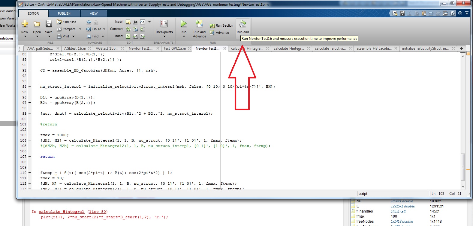
Matlab has a really nice timing-functionality for your code. You can access it simply by its icon in the Editor window, next to the basic Run-button. Just click it and wait for the results. Not that there’s any noticeable run-time difference compared to non-profiled running.

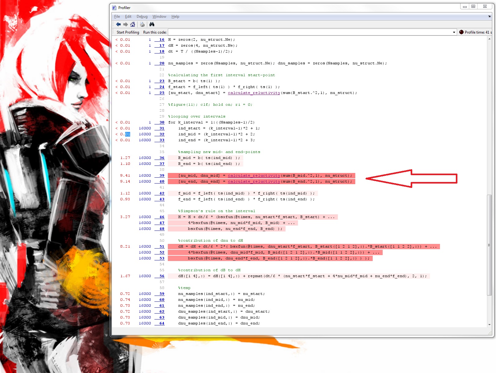
The window that pops up displays your code line-by-line, with the total time spent on executing each line displayed to its left. The slowest ones are even highlighted in different shades of red, the slowest being the darkest. Can’t get much easier, can it?

The first view is from the script that you started to profile. For me, it was simply some initialization stuff, plus a single call to the integration function I wanted to improve. Not very interesting then.

But, simply clicking any underlined function call in the profiler window shifts the view to that function (some pre-compiled low-level stuff excluded). And, you can move recursively deeper in the same way.

Below, you can find the results for my integration function. I’ll go through them in a moment, but let’s first consider some general guidelines about the profiler.

Indeed, the reverse Pareto principle usually holds quite strictly here. Something like 10 % of the code-lines often take more than 90 % of the total execution tim. Do something smart to those, and you’ll be an order of magnitude faster.

If they are function calls, move deeper to see what takes so long down there. If they are plain expressions – figure something out.

In my case, the total execution time was about 43 seconds. Of that, more than 18 was spent in the calculate_reluctivity function, and about 8 on the red-shaded long expression in the function body itself.

So, those three together take the majority of time. But what to do about them?

Well, we don’t need to do anything specifically about them yet. You see, each of those time-sapping lines was called a whopping 16 000 times during the function execution.

This number, here, brings me to my next point – which I’ll tackle in my next post.

-Antti

Matlab Speed Optimization – Case Example 1