Matlab speed tips continue. Remember to check the first part, well, first.
3. Vectorize. Then maybe vectorize some more.
Loops are generally somewhat slow in Matlab. They used to be much worse, but they’re still not stellar.
For this reason, you should try to write your code in vectorized form whenever possible. Vectorized means exactly what it sounds like – something that operates with arrays and vectors. No loops needed, that is.
Let’s say that you want to calculate ![]() ,
, ![]() ,
, ![]() , …,
, …, ![]() . In a lower-level language, you would write a loop with
. In a lower-level language, you would write a loop with ![]() running from 1 to 100, and compute
running from 1 to 100, and compute ![]() inside.
inside.
In Matlab, you can do this by writing (1:100).^2. The expression in the parentheses creates a vector with the entries running from 1 to 100, while the dot-notation corresponds to element-wise power of two. That’s a vectorized piece of code there. No loops, you see.
Okay, that was an exceedingly simple example. But, in practice, pretty much all built-in Functions in Matlab support vector input. Most can even be vectorized both row-wise and column-wise at the same time. Just check the documentation about the particularities of each, i.e. what actually happens in such a case.
Vectorization can often improve performance by a factor of 10. Neat.
Just a word of caution, though. Noticed how I recommended write vectorized code, not to vectorize it as an afterthought.
What I mean is that you should adopt a vector-based mindset early on. Trying to force loop-based code into vector format often is like trying to ram a square peg into a round hole. It can be done, but chopping the corners off the peg can take longer than expected, and the results are often horrible to read.
Example
Okay, let’s see how vectorization would help my code.
In the previous post, you saw how much time was spent on repeated function calls, one for each time-sample. Clearly not vectorized, right?
Well, yeah, but it’s still only a partial oversight on my part.
Remember that I needed to calculate the same type of integral at thousands of different positions ![]() ?
?
Yeah, I did vectorize that. Most of those array variables you see in the screenshot are in fact row-vectors (low but wide), with each entry corresponding to a different physical position in the problem.
But, I did not vectorize in the time-domain. I initially thought the number of time-samples would be much smaller than the number of positions. Obviously, I was wrong.
To speed things up, I implemented a partial vectorization in time. Meaning I computed all quantities at all positions, at several instants of time (but not all), and stored them in large matrices. Each row corresponding to a specific time-sample and so.
Then I let Matlab work its magic on those.
Due to memory limitations, I couldn’t handle all 32 000 time-samples simultaneously. Hence the term “partial vectorization”. I simply mean I operated on sets -chunks- of 1000 samples at a time. I still had a loop in my code, but its length was reduced from 32 000 to 32.
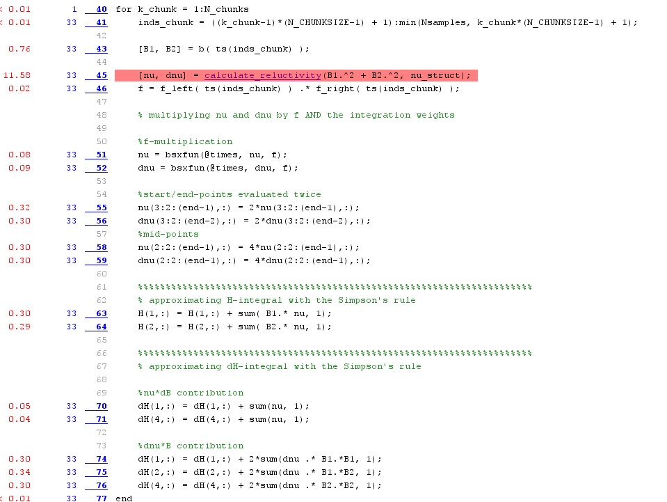
And the results prove it was good. Below, you can find the profiling results after this double vectorization.

As you can see, the earlier two function calls with 9 seconds each, have been replaced by one 11-second call. On okay-ish speed-up these. Additionally, all the plain expressions are much faster to evaluate, with no red shading visible beside that one function call. Indeed, what used to take eight seconds is now handled on three lines, about 0.3 seconds each.
All in all, this simple change brought the execution time to 15 seconds. Contrasting that the the earlier 43 seconds, that’s a nice improvement.
Also, note that the actual number of operations has been increased a bit. Indeed, the last sample of each 1000-long chunk is evaluated again as the first sample of the next chunk. (Because I’m lazy.) Despite this, the code is much faster. Kind of demonstrates the power of vectorization, right?
4. Go deeper and change something
Vectorization is indeed the most powerful and most general tip for Matlab. Well, that and not doing stupid shit.
Once that’s been sorted out, things get a lot more problem-specific. But, in general it’s a good idea to start going through the most time-consuming parts of code, and seeing if something could be done.
For me, that calculate_reluctivity function was obviously the worst offender after vectorization. Below, you can see what the Profiler had to say about its insides.

Indeed, most of the time is spent on the ppval function, a built-in function for evaluating piecewise polynomials.
You see, the term reluctivity refers to the inverse of permeability of each material. We need that in our problem, and its derivative too. However, for nonlinear materials, we don’t have any neat expression for it – only a set of measurement data. So, I thought it would be nice to initialize a set of spline interpolation polynomials for it, and then use those to quickly compute its value (and its derivative) at any flux density needed.
However, I noticed a weird thing – luckily. You see, splines are most commonly piecewise-defined third-order polynomials. But, at least in my version of Matlab, it was faster to use first-order interpolation instead. This was despite the fact that I had to increase the number of interpolation points to more or less match the accuracy of the third-order splines.
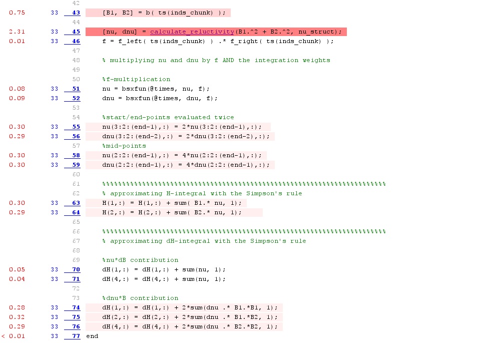
Indeed, with first-order interpolation, the calculate_reluctivity function only took 2.3 seconds, as you can see below. This brough the total execution time down to 6.1 seconds.

I want to point out one more thing: I could also have replaced the ppval function by my own implementation. Although the built-in functions in Matlab are generally quite fast, they are also very robust. They can handle several kinds of input, and recover from erroneous ones. However, you may know you need only a very specific kind of functionality for a tightly defined kind of data. In such cases, implementing your own special function is often justified and results in time-savings.
5. Go full HPC
My final tip is actually quite topical.
As you can see from the previous figure, quite simple operations now require the most of the time. The function calculate_reluctivity performs a very large number of very similar linear interpolations on a large array. The lightly-shaded plain expressions are also simple products and additions.
So, lot’s of repeated, independent, simple operations. If only we had a large number of simple processors to sort those out…
Wait, we do. The Graphic Processing Unit – GPU.
Luckily for us, Matlab can utilize the thousands of cores on the GPU quite nicely, for specific operations. Linear interpolation is among them, as are all elementary operations.
It isn’t even difficult to do. You just have to form a gpuArray of your data – moving it to your GPU memory. After that, Matlab utilizes its cores for your operations, whenever possible.
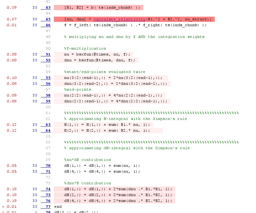
I let the results below speak for themselves.

Indeed, the reluctivity function call now finished in 0.67 seconds, rather than 2.31. The entire execution time has been shortened into 6.1 into 2.5 seconds.
Again, a word of caution. GPUs are generally fickle. Be careful. Also, the bus (PCIe, and similar) connection to the GPU is often the bottleneck. Hence, you probably need to have quite a hefty chunk of data – plus some simple-but-tedious operations on it – for the approach to yield any benefit. But, as I’ve just demonstrated here, it can still speed up your computations quite a bit.
Conclusion
I gave some general tips for speeding up you Matlab computations. I also took you through a real case example, optimizing my own Matlab function. Although some of my latter tips were very specific to my problem, I hope you still got something out of them. At least the general process is definitely worth following.
Indeed, it nicely ties up two of my favourite topics – the Pareto principle and the accumulated marginal benefit. Usually, most of your code speed-ups can obtained by fixing a few lines. That takes you 80 % of the time. Pareto there.
But after them, there’s no single easy way forward. Instead, there are several smaller ones, each quite insignificant on their own. But, once all of them have been fixed, you notice your program is now again much faster. Marginal benefit accumulated.
And yes, of course this entire process – improving your code again and again – is Kaizen if anything is.
Who knew programming could be so philosophical?
-Antti
Check out EMDtool - Electric Motor Design toolbox for Matlab.
Need help with electric motor design or design software? Let's get in touch - satisfaction guaranteed!
