Second-Order Finite Elements – Why, How, and When

Second-order finite elements - what and why

Hi all! You probably know by now that I’m collaborating a little with my colleagues on magnetomechanical analysis. So far, my input has mostly been limited to implementing FEA models in Matlab.

Well, one requirement that came up was the possibility to use second-order finite elements.

So, I thought I might write a little something on the topic. After all, the term may be unfamiliar to many. And besides, repetition is the mother of all lessons, or something like that.

Anyways, let’s begin with something simpler – first-order elements.

Basics of FEA – First-order elements

In magnetic FEA, we’re typically solving the field problem with the vector potential formulation. Meaning, the vector potential is the unknown quantity that is first solved by the computer.

Most commonly, first-order finite elements are used for this purpose. This simply means that the computer returns an approximate solution that is piece-wise linear.

You can check out this Wikipedia entry to get an idea of what piecewise linear means. It’s quite easy to understand in 1D – something simply consists of connected line segments. Things are a little more complex in two dimensions, but the figure below should illustrate things well.

Anyways, that’s what the approximate solution looks like. A collection of triangular surfaces, nicely continuous from element to element.

However, the vector potential is only a mathematical intermediate step – often we’re interested in the flux density .

By definition, the flux density is the curl of the vector potential. And since the curl is a derivative-type operator, the flux density will not be piecewise linear anymore.

Nope, we say it’s an order less continuous – piecewise constant. Meaning, it gets one value in one element, and another in the next one. This means that there can be a sharp jump on the boundary.

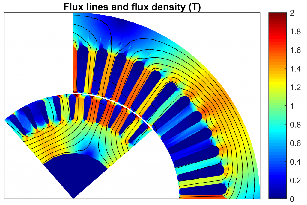
This is nicely evident from the flux plot below. The underlying mesh is so coarse that you can quite easily see the element borders, even though they haven’t been explicitly plotted.

Indeed, you can see how the magnitude of the flux density – the color scale – often jumps clearly from one element to the other. Also the direction of , illustrated with the black flux lines, undergoes a kink. There’s simply a corner in the flux line. Or lots of them.

Second-order elements

Alright, first-order elements yield a piecewise continuous solution. Or, in other words, a first-order solution. Meaning that the solution is a first-order polynomial of the x- and y-coordinates.

Now, you can probably guess what second-order elements do.

Indeed, they yield a second-order solution. Meaning, the vector potential can be expressed as a second-order polynomial of x and y.

Now, interesting things happen when we then compute the flux density . Again, the order is reduced by 1, meaning that the flux density is now a first-order function. Mind you, it is not automatically continuous from element to element. Not necessarily – that depends on the quality of the mesh.

But, it can be. Again, I think a figure should illustrate things nicely. Below, you can see the same flux plot, but computed with second-order elements.

Now, you can probably see some immediate differences. For instance, the color scale is much smoother. There are much fewer abrupt changes. Likewise, the flux lines behave more smoothly, too.

Alright, there are some jumps in the amplitude near the slot bottoms, but this is mostly a mesh quality issue. Meaning, it could benefit from a little refinement there.

Benefits and drawbacks

So, what’s the good and the bad in second-order elements?

Well, as hopefully became evident, second-order elements typically yield a better solution. That is, compared to using the same number of first-order elements.

However, the problem also has more unknowns, and takes longer to solve. So this is not an immediate win.

Instead, let’s think a little further. Imagine we used a denser first-order mesh, with more elements. Let’s say, enough elements that solving the problem took as long as our original second-order version. What would happen in this case?

Often, the second-order solution would still be better. Not always, but often.

Why this happens is related to the nature of finite element analysis. Let’s consider, for instance, the stator yoke in the above figure. You see that the flux density and flux line behave quite smoothly indeed. No sharp changes anywhere.

Nonsurprisingly, we say that the solution is smooth in that region. And mathematics tells us that smooth things can be better approximated be a few second-order elements compared to more first-order elements.

When to use which

So, when should we use which? That, unfortunately, often boils down to user experience. Or, you can take the systematic way and use any of the billion decision rules of hp-fem.

So, user experience. If you ask me, I’d always start with a first-order mesh. Just to see that the model works, and do any necessary rough adjustments.

Then, when the time comes for a more detailed analysis, I would switch on to second-order elements. Assuming the first-order solution “looks” smooth enough, of course. Meaning there not any obvious fine details that would benefit from a denser first-order mesh.

Conclusion

Second-order elements often yield a better and smoother solution compared to first-order elements. However, for initial model-building, first-order still rules.

-Antti

Second-Order Finite Elements – Why, How, and When